Support Vector Machine: A Machine Learning Algorithm

Support vector machine is an algorithm for supervised machine learning. This means the independent variables and the dependent or target variables are labeled as data to make a model train better. Support vector machine is used for regression as well as classification problems.

What happens in Support Vector Machine?

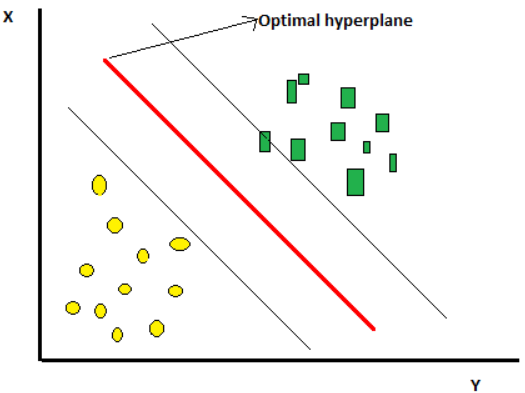
In a SVM algorithm all the data points are plotted in a n-dimensional space (when n denotes the features in the dataset). Each feature is plotted on specific coordinates in the n-dimensional space. After all the points are plotted, then the classification happens by determining a hyperplane that actually separates the classes or features.

Figure 1

The optimal hyperplane, or the SVM classifier, is something that has the maximum distance between two classes and best separates the classes.

How Does This Algorithm Work?

As we saw in the above figure, a hyperplane separates the two classes. Now the question arises, how can we be sure that we are choosing the right hyperplane? Lets see the below cases to understand the concept of hyperplane better:

Case1:

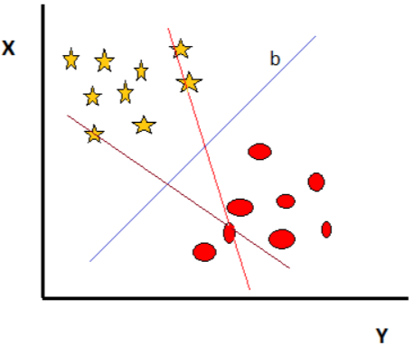
Figure 2

There are three hyperplanes in the above figure. The rule to find the appropriate hyperplane is “Choose the hyperplane that separates the star and circle better.” In this case hyperplane “b” is the correct hyperplane.

Case 2:

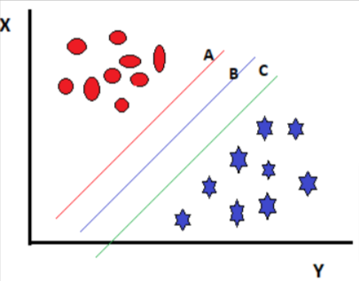
Figure 3

In the above case we have three hyperplanes and all are separating the classes well. Now, how do we select the best hyperplane?
The hyperplane that has the maximum distance from the closest data point in any of the classes is the correct hyperplane. This maximum distance is called a margin.

Case 3:

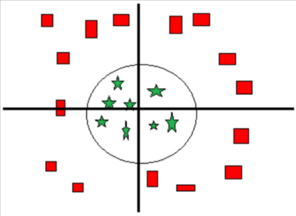
Figure 4

As in the above figure, there can also be the case when a straight line hyperplane cannot separate the two classes. In such cases the hyperplane can be a circle.

Support vectors are the vectors that are near to the boundary, the algorithm only works on the basis of support vectors. The points far away from the boundary do not have much effect on the algorithm.

SVM Hypothesis:

Figure 5
W designates weight. The SVM hypothesis can be explained as the distance between any data point and decision line or boundary.

Cost Function for One Training Sample:

-YLoss1(y, y^) – (1-y)Loss0(y,y^)

The left term denotes the loss when y equals 1 and the right term denotes it when y equals 0. Y^.
Loss function actually tells two things:

Y equals 1: when the distance or the hypothesis is greater than or equal to one, then loss will be zero. But if the distance is between zero and one, or any value less than one, then the loss will always be greater than zero and it will gradually go up.

Y equals 0: When the distance or hypothesis is greater than or equal to negative one, the loss will be zero. But if the distance is between negative one and zero, or a positive value, the loss will increase linearly and will be a positive value.

Comparison of SVM With Other Algorithms:

SVM generally has a high accuracy compared to other classifiers such as decision trees, logistic regression, etc. The execution time of SVM is short as compared to ANN. Additionally, it has better computation complexity in comparison to other algorithms.

Pros and Cons of SVM:

Advantages:

• SVM is extremely useful when we don’t have many clues about the data information or data isn’t distributed regularly.

• SVM doesn’t have overfitting, as there is a precise separation between the classes.

• It is used with high dimensional data.

Disadvantages:

• It cannot be used for a large volume of dataset. It takes a lot of training time for that.

• SVM hyper parameters are not easy to fine-tune.

• Selecting a good kernel is not easy in SVM.

Real Life Scenarios of SVM:

• SVM is used to detect people’s faces by separating the face and non-face parts using a square decision boundary.

• It is used in detecting handwritten characters.

• It is used in the medical field to detect cancer and other gene-related problems.

SVM Implementation:

Code:

1
2
3
4
5
6
from sklearn
import datasets
#loading the dataset
dfd = datasets.load_breast_cancer()
#Exploring the data
Print(“Features: “.cancer.feature_names)

Output:

1
Features: [‘mean radius’‘ mean compactness’‘ mean perimeter’‘ mean texture’‘ mean compactness’‘ mean area’‘ mean concavity’‘ mean concave points’‘ radius error’‘ mean symmetry’‘ texture error’‘ texture error’‘ area error’‘ compactness error’ perimeter error’‘ concave points error’‘ worst texture’‘ worst concavity’‘ symmetry error’‘ fractal dimension error’‘ smoothness error’‘ worst smoothness’‘ worst radius’‘ worst perimeter’‘ worst compactness’‘ worst area’‘ worst concave point’]

Code:

1
Print(“Labels: “, cancer.target_names)

Output:
Labels: [‘malignat’ ‘benign’]

Code:

1
2
3
4
5
6
7
8
9
10
11
12
13
14
15
16
17
18
19
20
21
#Splitting the data into train / test split
From sklearn.model_selection
import train_test_split
x_train, x_test, y_train, y_test = train_test_split(dfd.data, dfd.target, test_size = 0.3, random_state = 107)
#Generating the model
From sklearn
import svm
#Creating a svm classifier
cl = svm.SVC(kernel = ‘linear’)
cl.fit(X_train, y_train)
#Predict the response
for test dataset
y_pred = cl.predict(X_test)
#import scikit - learn metrics
from sklearn
import metrics
#Accuracy
Print(“Accuracy: “, metrics.accuracy_score(y_test, y_pred))
#Lets also check precision
Print(“Precision: “, metrics.accuracy_score(y_test, y_pred))
Print(“Recall: “, metrics.recall_score(y_test, y_pred))

Output:
Accuracy : 0.9649122807017544
Precision : 0.98113207547168981
Recall : 0.96269629629629629

We have got very good rates of accuracy, Precision etc. Its just a basic implementation , for actual real time datasets, we need to perform data cleaning, feature engineering, variables analysis and then apply the algorithm but I hope you got a good glimpse of SVM.