Comparison Networks

In this article, we look into sorting algorithms that use the comparison network model of computing to conduct several comparison operations at the same time. Comparison networks vary from RAM in two essential ways. For starters, they can only make comparisons. As a result, a counting sort algorithm can’t be implemented on a comparison network. Second, unlike the RAM paradigm, where operations are performed sequentially, or one after the other, activities in comparison networks can be performed simultaneously, or “in parallel.” This property, as we’ll see, enables the creation of comparison networks that order n values in sublinear time.

Introduction

Comparison networks are one of the types of sorting networks that constantly sort their inputs, therefore starting with comparison networks and their properties makes sense.

(a) A comparator with x and y inputs and x ′ and y′ outputs.
(b) A single vertical line representing the same comparator. The outputs x′ = 3 and y′ = 7 for respective inputs x = 7 and y = 3 are presented.

Wires and comparators are the only components of a comparison network. (a) part of the above figure shows a comparator, which has two outputs, x′ and y′ variables for the respective input variables x and y, performs the following function:

Because the graphical depiction of a comparator in (a) part of the above figure is too bulky for our needs, we’ll stick to portraying comparators as single vertical lines, as seen in the (b) part of the same figure. The smaller input value appears on the top output and the larger input value appears on the bottom output, with outputs on the right and inputs on the left. A comparator can thus be thought of as sorting its two input variables.

We’ll suppose that each comparator takes O(1) time to complete. To put it another way, we suppose that the interval between the emergence of input variables x and y and the generation of output variables x′ and y′ is constant.

Experimental Analysis

A wire is responsible for carrying data from one location to another. Wires can be used to link the input of one comparator to the output of another one, but they are either network input or network output wires otherwise. We’ll assume throughout this chapter that a comparison network has n input wires a1, a2,…, an, via which the variables to be sorted approach the network, and n output wires b1, b2,…, bn, which provide the network’s results. We’ll also refer to the variables on the output and input wires as the output sequence (b1, b2,…, bn) and the input sequences (a1, a2,…, an) respectively. That is, we refer to a wire and the payload it carries by the same name.

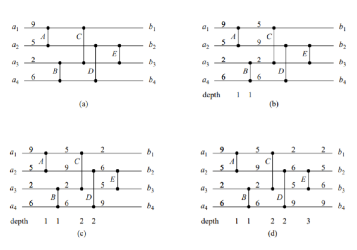
Figure (a) - A comparison network with four inputs and four outputs, which is actually a sorting network. The input variables presented on the four input lines occur at time zero.
Figure (b) - At time 1, the values displayed appear on the depth 1 output variables of comparators A and B.
Figure (c) - At time 2, the values shown appear on the outputs of comparators C and D at depth 2. The final variables for output wires b1 and b4 are now known, but not for output wires b2 and b3.
Figure (d) - At depth 3, the values depicted occur on the comparator E outputs at time 3. The final values for output wires b2 and b3 have been determined.

A comparison network is a collection of comparators connected by wires, as seen in the figure above. A comparison network with n inputs is represented as vertically stretched comparators with a group of n horizontal lines. A line represents a succession of different wires connecting various comparators, rather than a single wire. For example, the top line in the figure illustrates three wires:

• Input wire a1, which links to an input of comparator A.

• A wire linking an input of comparator C to comparator A’s top output to an.

• And output wire b1, which arrives from comparator C’s top output.

Each input of the comparator is linked to one of the network’s n input wires a1, a2,…, an or the output of this other comparator. Similarly, each comparator output is linked to a wire that is any one of the network’s n output wires b1, b2,…, bn, or another comparator’s input. The most critical requirement for interlinking comparators would be that the graph be acyclic; that is if we trace a path from one comparator’s output to another’s input to output to an input, and so on, the path we trace shouldn’t ever cycle back on itself and pass through the same comparator twice.

Conclusion

A sorting network is called a comparison when the network in which the output sequence for each input sequence is uniformly increasing (i.e., b1, b2 … bn). Of course, not all comparison networks are also sorting networks, but the network represented in the above figure is. To see why, consider that after time 1, either the top result of comparator B or the top result of comparator A has provided the least of the four input values. As a result, it should be on top of the comparator C output after time 2. After time 2, the bottom result of comparator D has provided the highest of the 4 input values, according to a symmetrical argument. All that’s left is for comparator E to check if the two middle values are in the right output places at time 3, which it does.

A comparison network is similar to a process in that it describes how comparisons should be made, but it differs in that its physical size is determined by the number of outputs and inputs. As a result, we’ll be talking about the “families” of comparison networks. The purpose of this chapter, for example, is to create a SORTER family of sorting networks that is efficient. The number of inputs and the family name is used to identify a specific network within a family (which equals the number of outputs). SORTER[n], for example, is the name of an n-output, n-input sorting network of the SORTER family.

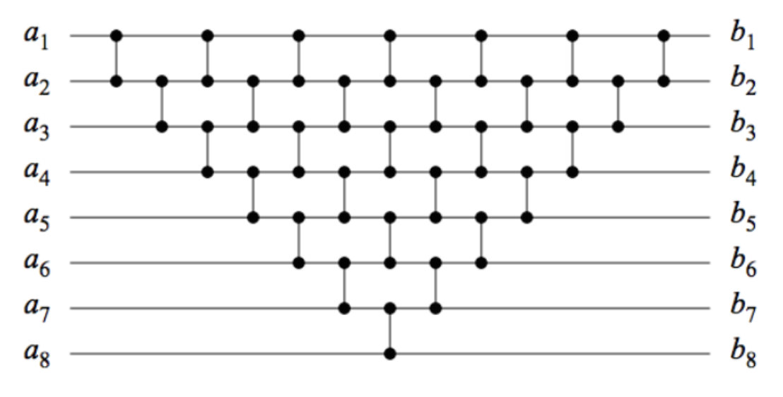
The above figure represents a comparison network based on insertion sort.