Overview of Gradient Boosting Algorithms

Overview of Boosting Algorithms:

Boosting algorithms are supervised learning algorithms that are mostly used in machine learning hackathons to increase the level of accuracy in the models. Before moving on to the different boosting algorithms let us first discuss what boosting is.

Suppose you built a regression model that has an accuracy of 79% on the validation data. Then you decide to implement one more model by building a decision tree and K-NN models on that data itself. The above respective models give you an accuracy of 82% and 66% on the validation set.

We know that the above three models all work in different ways. Regression is trying to capture the linear relation in the data, while KNN is classifying the data, etc.

Instead of using just one model on a dataset, lets combine the models and apply them on the dataset, taking the average of the predictions made by all the models. If we do this, we will be capturing extra information from the dataset.

The basic idea behind this approach is ensemble learning. So what about boosting?

Boosting is one method that uses the idea of ensemble learning. Boosting algorithms merge different simple models to generate the ultimate output.

Now for an overview of various boosting algorithms:

Gradient Boosting Machine (GBM):

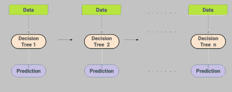
A GBM combines distinct decision trees’ predictions to bring out the final predictions. Now the question may pop into your mind, how do these dissimilar decision trees capture the different information from the data? Let’s understand how it happens.

The nodes in each decision tree take a distinct subset of the features for picking out the best split. This signifies that actually these decision trees aren’t all identical and therefore they are able to capture distinct signals from the data.

Moreover, every tree considers the errors made by the previous decision tree. Hence, every successor tree is made on the error of the previous tree. Below is the representation of GBM.

Figure 1

XGBM or Extreme Gradient Boosting Machine:

XGBM is just another version of GBM. The working methods of both the algorithms are very similar. Here also the trees are built one after the other, correcting the mistakes of the previous trees.

However, there are a few differences as follows:

• Extreme gradient boosting machine consists of different regularization techniques that reduce under-fitting or over-fitting of the model and increase the performance of the model.

• It also performs parallel preprocessing of each node, which makes it more rapid than GBM.

• Moreover, while using XGBM we don’t need to think of imputation of missing values, this model takes care of it. It learns on its own whether these values should be in the right or left node.

Light GBM

Light GBM  is growing in demand due to its efficiency and fast speed. It can handle a large volume of data with great ease. However, light GBM  does not go well when the data points are small in number.

Rather than a level-wise growth of the nodes of the tree, light GBM follows a leaf-wise growth. When a root node is split into two the next split depends upon which between two nodes has a higher loss, and that node is selected for the other split.

This algorithm works well with large volumes of data due to this leaf-wise split.

Figure 2

Catboost:

This algorithm is basically for handling the categorical features in a dataset. Most machine learning algorithms work on numerical data better. The essential preprocessing step in every algorithm is to convert categorical features into numerical variables.

Unlike other algorithms, catboost can handle the conversion of categorical features into numerical internally.

The approach of converting categorical features into numerical features is as follows:

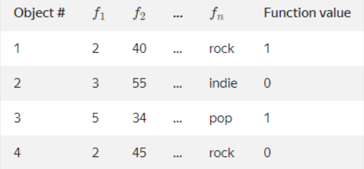
• This algorithm accepts various model values and object properties as input.

Figure 3

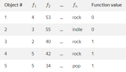
• Many permutations are created for these rows/data randomly.

Figure 4

• This is the formula used to convert categorical into numerical features

Avgtarget =  countInclass +prior/ totalcount + 1

• CountInclass is the count of number of times label value =1 for the specific objects with current categorical variable value.

• Prior is the prior value for the numerator. Starting parameters determine it.

• Totalcount is the total count of objects (until the current one) that have a categorical variable value matching the current one.

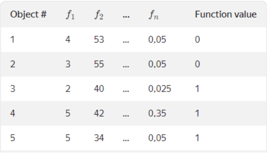
• Here in this case, b = [1:,3] includes values “rock”, “indie”, “pop”.  Prior is set to 0.05.

The result will be something like this.

Figure 5

Boosting Algorithms in Comparison to Other Algorithms:

• Boosting algorithms compared to random forests: In boosting algorithms every tree is built one at a time, whereas random forests build each tree independently.

• XGBoost is comparatively more stable than the support vector machine in the case of root mean squared errors.

Advantages and Disadvantages of Boosting Algorithms:

Advantages:

• Boosting algorithms follow ensemble learning, therefore it’s simple to make an interpretation of its prediction.

• It is irrepressible to overfitting.

• It has an implicit feature selection method.

Disadvantages:

• It is difficult to scale this algorithm as every estimator is dependent on its predecessor.

• It is somewhat slower to train compared to algorithms like bagging.

Real Life Applications of Boosting Algorithms:

• Boosting algorithms’ main real-life application is to merge different algorithms to increase accuracy or to make stronger predictions.

• Boosting algorithms are used in hackathons or competitions to increase the accuracy of the models.

I hope the concept of boosting algorithms is now clear to you.